David silver’s reinforcement learning lecture 4

2 minute read

Model-Free Prediction

이제부터는 model을 모르는 상황에 대해 최적의 value function을 찾는다.

1. Monte-Carlo Reinforcemnet Learning

MC는 episode들을 직접 경험하면서 학습하는 방법이다.

episode가 끝나면 return의 평균으로 value를 정한다.

단, MC는 episode가 있고 끝나야만 적용 가능하다는 단점이 있다.

Monte-Carlo Policy Evaluation

여기서 empirical mean return은 직접 episode를 경험하고 얻은 return들의 평균값을 의미한다.

단, 여기서 모든 state를 방문한다는 가정이 있어야 적용할 수 있는 방법이다.
- First-Visit Monte-Carlo Policy Evaluation
  
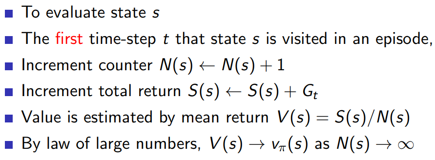
  first-visit은 어떤 state에 처음 방문한 경우만 고려하는 방법이다(재방문은 무시).
  
  state의 갯수(방문한 횟수)가 커지면 value가 최적의 상태로 수렴하게 된다.
- Every-Visit Monte-Carlo Policy Evaluation
  
  every-visit은 state에 재방문한 경우도 포함하는 방법이다.
- Incremental Monte-Carlo
  - Inremental mean
    
    평균을 구할 때 위와 같이 변형하면 이전 평균에다가 새로운 값이 들어오면 바로 update를 할 수 있게 된다.
    
    그냥 일반적으로 구하는 평균은 값을 전부 다 기억하고 있어야 하는데, large problem의 경우 메모리를 많이 사용.
    
    이 방식으로 하면 이전 값들을 전부 다 기억할 필요없이 새로운 값이 들어올 때 바로바로 업데이트 가능. 즉, 메모리를 아낄 수 있다.
  - Incremental Monte-Carlo Updates
    
    Incremental mean 방식으로 value를 업데이트한다.
    
    non-stationary problem이란, action을 취할 때마다 MDP가 바뀌는 문제를 말한다. 따라서, 이 경우에는 이전의 값들의 중요도가 떨어지니까 alpha로 줄여준다.

2. Temporal-Difference Learning

TD 또한 MC와 마찬가지로 episode를 경험하여 학습하는 방법이다. 그래서 TD도 model-free에 적용 가능하다.

단, episode가 끝나고 난 뒤에 update하는 MC와는 달리, TD는 episode가 끝나기 전인 불완전한 상태로, 즉, bootstrapping(추정치를 추정치로부터 업데이트)으로 학습한다.

episode가 끝나고 얻은 return(G)으로 value를 업데이트하는 MD와 달리, TD는 바로 다음 state에서의 추정치를 통해 업데이트를 한다.

Driving Home Example

이 예시에서 MC는 예측 경과 시간이 집에 도착(terminal state)하고 update 되는 반면에, TD는 다음 state의 value로 update되는 것을 볼 수 있다.
Characteristics of MC and TD
- MC
  - update를 하려면 episode가 끝날 때까지 기다려야 한다.
  - 따라서, episodic(terminating) environments 경우에만 적용 가능하다.
  - episode가 끝난 뒤 얻는 return으로 업데이트를 하는데, 이는 unbiased 이다.
  - Return은 많은 random actions으로부터 얻기 때문에 variance가 크다.
  - 초기값에 전혀 민감하지 않다.
  - Markov property를 이용하지 않는다.
- TD
  - 매 step마다 업데이트 할 수 있다.
  - TD는 continuing(non-terminating) environments 에도 적용 가능하다.
  - TD target은 biased 이다. (대부분 biased여도 최적으로 수렴한다고 한다.)
  - TD target은 한 번의 random action으로 얻기 때문에 variance가 작다.
  - 초기값에 민감하다.
  - Markov property를 이용한다.
- Unified view of Reinforcemnet Learning
  
  TD는 sampling을 하고, bootstrapping을 한다.
  
  MC는 smapling을 하고, bootstrapping을 하지 않는다.
  
  DP는 sampling을 하지 않고, bootstrapping을 한다.
n-Step TD

TD target을 바로 다음 state가 아니라 n-step 이후로 설정해도 된다. 여기서, n이 커질수록 TD는 MC에 가까워진다.
- n-Step Return
  
  n-step 이후에 설정한 return을 수식으로 나타낸 것이다.
Forward-view TD(λ)

TD(λ)는 1부터 n까지의 모든 return을 결합한 것이다. 이때, geometric mean으로 λ-return을 얻는다.

n쪽으로 갈수록 (1-λ)에 의해서 weight가 줄어든다. (λ는 0과 1사이의 값)

forward-view 방식은 MC와 마찬가지로 episode가 끝나야 계산할 수 있다. 즉, TD의 장점이 사라지게 된다.
Backward-view TD(λ)

Update online, every step, from incomplete sequences
- Eligibility Traces
  
  Eligibility trace는 최근에 발생한 state와 빈번하게 일어난 state 모두를 고려하여 계산한 것이다. state가 발생할 때마다 1을 더해주고 시간이 지날수록 조금씩 감소시키면 frequenct heuristic과 recency heuristic 둘 다를 만족시킬 수 있다.
  
  여기서 gamma는 0과 1사이의 값이다.

TD-error와 dligibility trace를 통해 value를 업데이트한다.

TD(0)

backward-view 식에서 λ=0을 대입하면 TD(0)랑 똑같아진다.
TD(1)

offline update일 경우에는 forward-view와 backward-view가 일치한다고 한다.

λ=1일 경우에는, MC랑 같아진다.

증명은 아래와 같다.